What is the optimal size, shape and number of plots for field trials?

All about plots

When designing the physical aspects of a crop experiment, there are many choices to be made surrounding plots for the researcher to contend with:

• How many plots should my experiment have?
• What size and shape should my plots be?
• How can I prevent interactions between plots?

Luckily for researchers today there are straightforward solutions to these problems and QuickTrials can help to implement them.

How to prevent interactions in field trials

Number of plots

The number of plots in an experiment is determined solely by the number of treatments that are being tested, and the number of times that each of those treatments is replicated. The relationship is simple: the total number of plots is the number of treatments multiplied by the number of replications.

However, despite this apparent simplicity, there is an underlying mathematical relationship (Hathaway, 1963) connecting the number of replications, the plot size (area), with the ability to detect statistical differences. The derivation of this relationship relies on using direct observations from previous experiments, such as yield, to calculate an index of variability unique to each field for a fixed plot size. The index of variability ranges from 0 to 1, with 0 being a completely heterogeneous (varying) field, and 1 a completely homogeneous field (uniform).

Assuming that the number of treatments in the experiment is fixed, to determine the number of replications required the researcher must have an idea of the smallest difference between treatments that must be measurable, given the underlying experimental error. This is known as the detectable difference and is usually reported as a percentage of the mean of an observation, such as yield.

For example, if the researcher needs to be able to detect a 15% difference in yield between treatments that have plots of 20m2 , reading from the chart in Figure 1, they will need at least 6 replicates to achieve this.

The explanation and calculation of the index of variability and the corresponding relationship between plot size, replications and detectable difference is too detailed to be explained in this article but interested readers may follow the references at the end of the article.

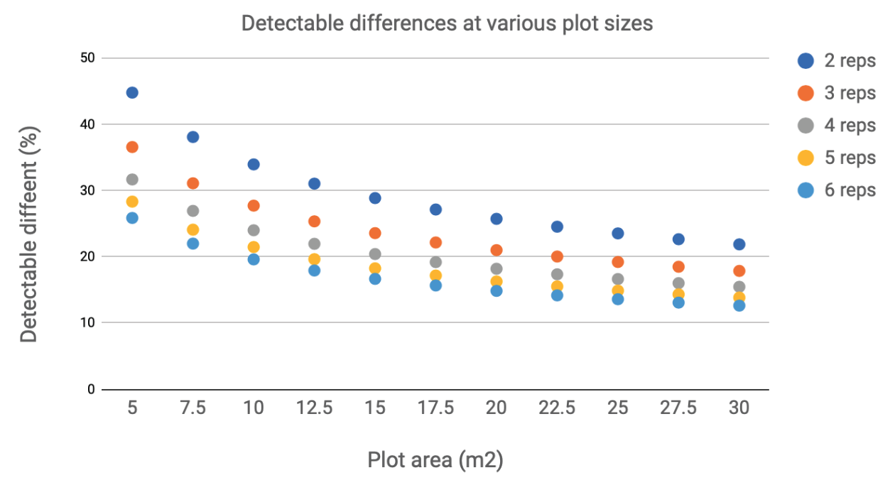
Figure 1: Relationship between detectable difference, number of replicates and plot size

Plot size

In theory, it is possible to mathematically calculate the economically optimum plot size, as formulated by Smith (1938) which is:

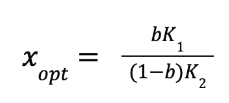
Where b is the index of variability, calculated on a fixed plot size, K₁ is a cost that is independent of plot size, K₂ is a cost dependent on plot size, and xopt is the factor that when multiplied by the plot size associated with the index of variability, calculates the most economical plot size for that field.

In practice however, it is often the case that other constraints limit the freedom of the researcher to choose their plot sizes. For example, when developing new varieties, a breeder will work with a range of plot sizes, from plants grown from a single seed in pots, to small nursery plots grown from the seed of a single plant, to large yielding plots designed to produce seed in quantity. Generally, the later the stage of the research, the larger the plots.

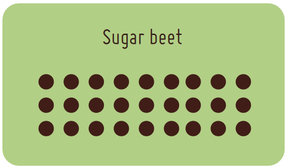
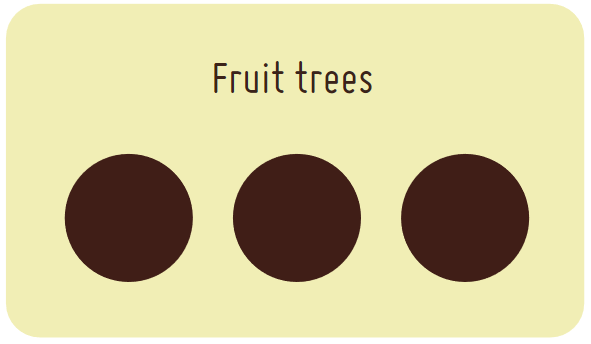
The species of crop is also a major factor which influences the plot size. The plots must contain enough plants to account for the experimental error but also leave enough room for the plants to grow to their potential without overcrowding. Cereals like wheat and barley can make use of more compact plots due to the large number of plants per unit area whereas crops planted in rows, such as sugar beet for example, need larger plots to accommodate a suitable number of plants. Experiments on fruit producing trees again require even larger plots to allow for the adequate space between trees.

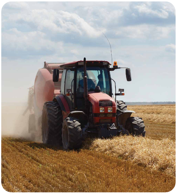
The other major determinant of plot size is the machinery used to implement the trial. In practice, this will, at the very least, determine the minimum size of the plot. Most plots are typically sown or planted with machinery as well as having their treatments applied with fixed-size equipment. Therefore, the smallest plot size is usually that of the largest piece of equipment involved in the experiment. In certain types of experiments, such as farming systems research, plots can become very large as they make use of commercial farming equipment. In these cases, it is not uncommon for plots to be as large as 50m x 50m to allow for machinery application overlaps.

Plot shape

Ideally the shape of a plot should be as compact as possible to minimise the impact of any underlying soil variability. In practice, thin, rectangular plots are more convenient for sowing, spraying, and harvesting. In fact, as the crop research industry has matured and more mechanisation has been possible, plot sizes for certain crops, like wheat and barley, have developed to a standard width of around 2 metres, with varying lengths depending on the purpose of the experiment.

Plot orientation

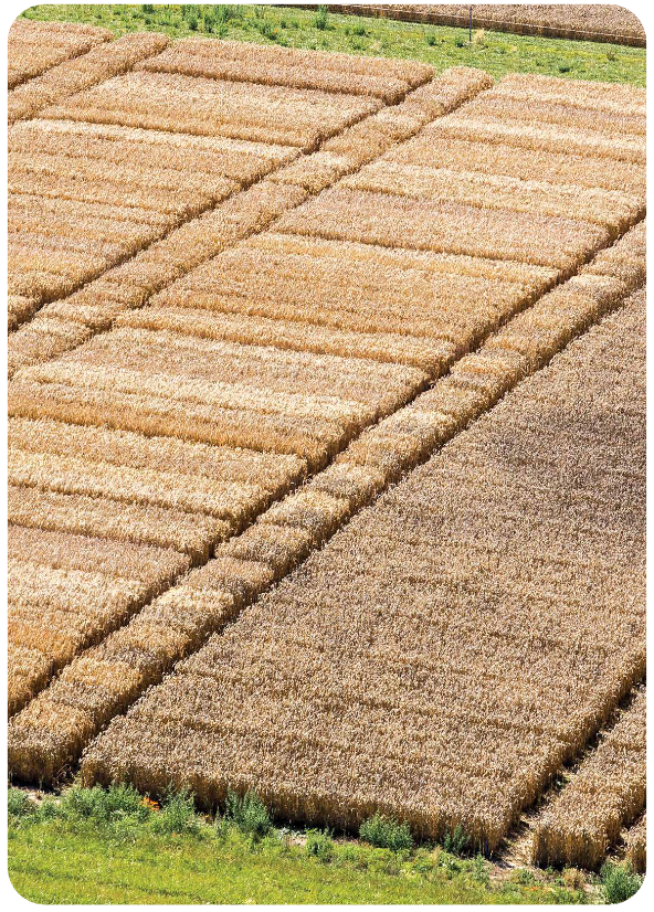
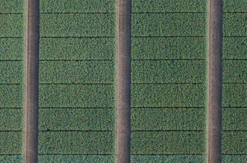
Assuming a typical rectangular plot shape, plots should be oriented with the long edge parallel to any lines of variation. Since most experiments are usually located in commercially managed fields, much of the potential variation that plots may experience comes from field operations like cultivation, sowing and spraying. It follows that plots should be oriented perpendicular to the direction of work (i.e. perpendicular to the field tramlines, Figure 2), as the potential gradient of variability is likely to be along the length of the equipment (e.g. blocked nozzle or coulter).

Orienting the plots parallel to the tramlines also has an impact on the plot length. Again, due to standardisation of farming machinery, tramlines are usually spaced 24m apart (although 30m is becoming more common with the trend for larger equipment). Plots may then have possible lengths of 6, 12, or 24 metres, which allows them to be evenly placed between the tramlines. This fact is also leading to the standardisation of plot lengths within the crop research community.

Illustration showing plot orientation in field trials

Figure 2: Rectangular plots are arranged to fit between tramlines.

Edge effects and plot borders

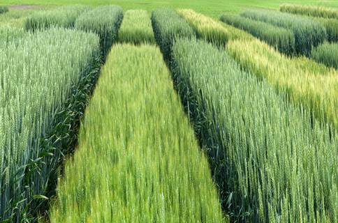
Adjacent plots usually have small unplanted areas between them often referred to as wheelings or alleys, (Figure 3). These spaces are useful as it allows for people and equipment to travel freely around the experiment without damaging the plots. They also clearly mark out the plot areas to help maintain plot separation during important activities like harvesting. However, these spaces can cause issues where plants at the edge of the plot grow much larger than plants within the plot due to less competition for water, nutrients, and sunlight. This is known as an edge effect and the solution is to either avoid taking any observations at the edges of the plots, or planting extra plants to act as a buffer to the plot, usually called discard or guard rows. In the case of the former, plot edges are often removed (e.g. mown) before the plot is harvested.

In the same way the edge effects in the plot appear through lack of competition, sometimes adjacent plots can compete in ways which would bias the experiment. For example, if a researcher has a maize variety trial where some varieties are very tall and some are very short varieties, a tall variety will outcompete a short variety for sunlight.

There are two solutions available to the researcher in this case. Firstly, they could adjust the trial design so that incomplete blocks are grouped by variety height, meaning that short varieties do not appear next to tall varieties. Secondly, they could insert a mixed guard row between each plot so that any competition effects can be safely ignored.

Figure 3: Wheelings or alleys between plots

Conclusion

As we have seen, there are many factors in choosing the right plot size and shape: crop, stage of the research, equipment to be used and so on. Fortunately, as the industry has matured, standards and consistent methods have emerged to allow researchers to design experiments efficiently and economically within these constraints.

The QuickTrials software can accommodate many different trial set-ups, making it easy to define the number of plots, size and layout to avoid plot interactions and obtain the optimal results for your trial.

References

Hathaway, W. H., 1963. Convenient plot size. Agronomy Journal 53:279-280.
Smith, H. F., 1938. An empirical law describing heterogeneity in the yields of agricultural crops.
Journal of Agricultural Sciences 28:1-23.